This tutorial builds directly on Tutorial 2. We'll use the same two datasets, the 2015 NYC Street Tree Census and the census block geopackage, and repeat the same spatial join. The difference is what we do before the join. Instead of just counting trees, we'll estimate two ecological services each tree provides: stormwater interception and CO₂ sequestration. Then we'll aggregate those benefit estimates spatially to see which neighborhoods are getting the most (and least) out of the city's urban forest. At the end, we will run the estimate forward in time.
In the vocabulary of this class, last week's map was a record. This week we apply a rule, which is a model. Then we run the rule, or give it time, which is a simulation.
NYC Parks puts a number on these services for every street tree on its Tree Map. The numbers come from i-Tree Streets, a model from the USDA Forest Service. We will follow the same method, as closely as a notebook allows. i-Tree Streets' assumptions for the Northeast are written down in the Northeast Community Tree Guide (McPherson et al. 2007, Appendix 3), and the equations it uses are published in the Urban Tree Database (McPherson, van Doorn and Peper 2016). Every number below comes from one of those two reports unless I say otherwise.
A note: this is a best approximation of NYC Parks' published "ecological benefits of street trees," using what is published about the i-Tree Streets app. I'll name what is coming from where, and when I am making educated guesses. As you'll see below, we're going to get mildly lost in some coefficients and crown diameter's for a bit, but stay with it and just try to understand the general logic.
You need three files. The first two are the same ones from Tutorial 2. The third is in the course folder, under the name of this tutorial:
2015_Street_Tree_Census_subset_um.csvnycb2010_um.gpkgqueens_tree_equations.csv
Setup
We will use Google Colab again this week. If you would rather run this on your own computer, the setup is in Running Python on Your Own Computer; the code is the same apart from the upload step.
Same imports as Tutorial 2, with numpy added. We need it for the logarithms in the equations.
from google.colab import files

import numpy as np
import pandas as pd
import geopandas as gpd
import altair as alt

# Altair defaults to a 5,000-row limit; disable it since our dataset is larger
alt.data_transformers.disable_max_rows()
Upload the three files:
uploaded = files.upload()
Step 1: Load the data
Load the street tree CSV exactly as in Tutorial 2. The columns we'll use most are tree_dbh (diameter at breast height, in inches), spc_latin (species name), and the lat/lon coordinates.
df_StreetTree = pd.read_csv('/content/2015_Street_Tree_Census_subset_um.csv')

# Preview the data
df_StreetTree.head()
Before calculating anything, let's check the status column. The census records stumps and dead trees as well as living ones. Stumps have a DBH of 0, and dead trees have a diameter but no species. Neither catches rain or takes up carbon, so we keep only the living trees:
# Count living trees, dead trees and stumps
print(df_StreetTree['status'].value_counts())

# Keep only the living trees. .copy() makes this a table of its own, so pandas doesn't warn when we change it
df_StreetTree = df_StreetTree[df_StreetTree['status'] == 'Alive'].copy()
We should also check the range of the diameters. Run df_StreetTree['tree_dbh'].describe(). The maximum in this subset is 228 inches, which is a trunk nineteen feet across, and is a data entry error. We will replace anything above 60 inches with NaN, which means "Not A Number", so the equations return nothing for that tree instead of a wrong value. The 60 inch cutoff is my choice.
# One record claims a 228-inch trunk. Treat anything over 60 inches as a data entry error.
df_StreetTree.loc[df_StreetTree['tree_dbh'] > 60, 'tree_dbh'] = np.nan
Step 2: Match each tree to a species from Queens
In 2005 the Forest Service measured the trunk, height and crown of 910 street trees of 21 species in Queens, and dated 150 of them from tree cores. From those measurements they fitted equations that predict the size of a tree of each species from its trunk diameter. Fitting an equation to measurements like this is called a regression, and every equation in the file we load below is a regression. Queens is i-Tree's reference city for the whole Northeast, so these are the equations behind Parks' numbers (Northeast Community Tree Guide, pp. 92-93).
queens_tree_equations.csv has five equations for each of the 21 species, copied from the Urban Tree Database. Each row is one equation for one species, with its coefficients in a to d:
utd = pd.read_csv('/content/queens_tree_equations.csv')
utd.head(10)
Now give each tree in the census one of the 21 species. About three quarters of the trees in our subset are one of the 21. For the rest, we use a species of the same genus (a white oak is treated as a pin oak), and anything left over is treated as a honeylocust, the most common tree in the subset. This ovbiously isn't the most accurate choice, but is a necessary simplification to keep things straightforward.
# The 21 Queens species, by scientific name
species = dict(zip(utd['scientific_name'], utd['SpCode']))

# For a species that isn't one of the 21, the most common Queens species of the same genus
same_genus = {'Acer': 'ACRU', 'Quercus': 'QUPA', 'Tilia': 'TICO', 'Ulmus': 'ULAM',
              'Prunus': 'PRSE2', 'Malus': 'MA2', 'Fraxinus': 'FRPE', 'Pinus': 'PIST'}

def match_species(latin):
    if pd.isna(latin):
        return 'GLTR'
    if latin in species:
        return species[latin]
    first_two = ' '.join(latin.split()[:2])   # 'Gleditsia triacanthos var. inermis' -> 'Gleditsia triacanthos'
    if first_two in species:
        return species[first_two]
    # Anything else is treated as a honeylocust (GLTR), the most common tree in the subset
    return same_genus.get(latin.split()[0], 'GLTR')

df_StreetTree['SpCode'] = df_StreetTree['spc_latin'].map(match_species)
df_StreetTree['SpCode'].value_counts()
Step 3: The equations
The Urban Tree Database uses six kinds of equation, listed in Table 3 of the report. The form column says which one a row uses.
A function that evaluates one equation. x is the input (trunk diameter in centimeters, or age in years). In the log-log and exponential forms, c is the equation's mean squared error.
def equation(form, a, b, c, d, x):
    if form == 'lin':      return a + b*x
    if form == 'quad':     return a + b*x + c*x**2
    if form == 'cub':      return a + b*x + c*x**2 + d*x**3
    if form == 'loglogw1': return np.exp(a + b*np.log(np.log(x + 1) + c/2))
    if form == 'loglogw2': return np.exp(a + b*np.log(np.log(x + 1)) + np.sqrt(x)*c/2)
    if form == 'expow1':   return np.exp(a + b*x + c/2)
A function that applies one kind of equation to every tree, using each tree's own species. The dry weight equation takes height as well as diameter, and has the same form for every species. x_max is only set on the age equation: it is the largest tree that equation should be used for, so a bigger tree is treated as that size when we estimate its age.
def predict(what, sp, x, height=None):
    out = np.full(len(x), np.nan)
    # This loops over the species, since each species has its own coefficients
    for code in np.unique(sp):
        # This is the one row of the equations file for this species and this equation
        row = utd[(utd['SpCode'] == code) & (utd['predicts'] == what)].iloc[0]
        i = (sp == code)
        # This caps the input at x_max, the largest tree the equation is meant for
        xi = x[i] if pd.isna(row['x_max']) else np.minimum(x[i], row['x_max'])
        if what == 'dry_weight_from_dbh_height':
            # This estimates wood volume from diameter and height, times the wood's density (d)
            out[i] = row['a'] * xi**row['b'] * height[i]**row['c'] * row['d']
        else:
            # This is every other equation, using the forms in equation() above
            out[i] = equation(row['form'], row['a'], row['b'], row['c'], row['d'], xi)
    return out
Go ahead and copy both cells into your notebook before we proceed.
Step 4: Stormwater interception
Purportedly, one of the most economically significant services street trees provide is intercepting rainfall before it reaches the ground. NYC's stormwater drainage and sewage system share the same pipes, and heavy rainfall onto impervious surfaces cause CSO's, or "Combined Sewer Overflow", which is why it is typically not recommended to head to the beach after heavy rainfall. Trees reduce the volume of stormwater entering the system.
First we need the size of each tree's canopy. The goal here is crown projection area, the footprint of the canopy as seen from above, modeled as a circle. The crown diameter comes from the species' equation.
i-Tree estimates interception by simulating a year of hourly rainfall at JFK airport, filling and emptying each crown's leaves storm by storm. That is too much for this notebook. Instead we take one number from a field study: Xiao et al. (2000) put rain gauges above and below two trees in Davis, California for two winters, and found that the crown of a Callery pear caught about 15% of the rain falling on it. (A cork oak in the same study caught 27%.) We apply that 15% to the rain over each crown's footprint. For the rain, we use the same year i-Tree used for the Northeast: 41.0 inches at JFK in 2000 (Northeast Community Tree Guide, p. 100).
rain_m = 41.0 * 0.0254          # JFK airport, 2000 (Northeast Community Tree Guide, p. 100)
interception_fraction = 0.15    # a Callery pear in Davis, CA (Xiao et al. 2000)

def stormwater_gal_yr(sp, dbh_cm):
    # Crown diameter (m) from trunk diameter (cm). Very small trees can come out below zero; count those as zero.
    crown_m = np.maximum(predict('crown_diameter_from_dbh', sp, dbh_cm), 0)
    # Crown projection area (m²), modeled as a circle
    crown_area_m2 = np.pi * (crown_m / 2) ** 2
    # Rain over the crown (m³) x the share the crown catches, in gallons (1 m³ = 264.17 gallons)
    return crown_area_m2 * rain_m * interception_fraction * 264.17

sp = df_StreetTree['SpCode'].to_numpy()
dbh_cm = df_StreetTree['tree_dbh'].to_numpy() * 2.54

df_StreetTree['stormwater_gal_yr'] = stormwater_gal_yr(sp, dbh_cm)

print(f"Total stormwater intercepted per year: {df_StreetTree['stormwater_gal_yr'].sum():,.0f} gallons")
print(f"Median per-tree interception: {df_StreetTree['stormwater_gal_yr'].median():,.0f} gal/yr")
The median tree comes out at about 1,450 gallons a year. The Parks department average for the 2015 census is 1,376 gallons per street tree citywide (TreesCount! 2015). So we're in the ballpark of the correct number, but that number is also over an average for the full city, instead of this subset.
Step 5: CO₂ sequestration
Trees sequester carbon as they grow, converting atmospheric CO₂ into wood. We estimate how much CO₂ each tree stores now, how big it will be next year, and take the difference. The steps are the ones in Appendix 5 of the Urban Tree Database (p. 73):
- Height from trunk diameter, from the species' equation
- Dry weight of the wood above ground, from diameter and height
- Multiply by 1.28 to add the roots, by 0.5 because about half of dry wood is carbon, and by 3.67 to convert carbon to CO₂
For growth, the database has two more equations per species: the tree's age from its diameter, and its diameter at each age. We estimate each tree's age, then add one year's growth from the diameter-at-age curve.
def co2_stored_kg(sp, dbh_cm):
    height_m = predict('height_from_dbh', sp, dbh_cm)
    dry_weight_kg = predict('dry_weight_from_dbh_height', sp, dbh_cm, height_m)
    return dry_weight_kg * 1.28 * 0.5 * 3.67   # roots, carbon, CO2 (Urban Tree Database, p. 73)

def grow_one_year(sp, dbh_cm, age):
    # How much a tree of this species and age thickens in a year. Past the end of the curve, it stops.
    step = predict('dbh_from_age', sp, age + 1) - predict('dbh_from_age', sp, age)
    return dbh_cm + np.maximum(step, 0)

age = np.maximum(predict('age_from_dbh', sp, dbh_cm), 0)
df_StreetTree['age'] = age
df_StreetTree['co2_seq_kg_yr'] = co2_stored_kg(sp, grow_one_year(sp, dbh_cm, age)) - co2_stored_kg(sp, dbh_cm)

# Dollar value: $0.00334 per pound of CO2 (Northeast Community Tree Guide, Table 18)
# To try another price, swap it in for 0.00334:
#   $0.0231 per pound of CO2 ($51 a metric ton, Biden admin, 2021)
#   $0.0862 per pound of CO2 ($190 a metric ton, EPA, 2023)
df_StreetTree['co2_value_usd'] = df_StreetTree['co2_seq_kg_yr'] * 2.2046 * 0.00334

print(f"Total CO₂ sequestered per year: {df_StreetTree['co2_seq_kg_yr'].sum():,.0f} kg")
print(f"Total CO₂ value per year: ${df_StreetTree['co2_value_usd'].sum():,.0f}")
print(f"Median per-tree sequestration: {df_StreetTree['co2_seq_kg_yr'].median():.1f} kg CO₂/yr")
The $0.00334 a pound (about $7 a metric ton) is the price in the Northeast guide, and it is also the price on the Parks Department Tree Map. It is an estimate of the damage a ton of CO₂ does, taken from the average of a 2003 survey of such estimates (Pearce 2003). The Biden Administration's figure for the "social cost of carbon" was $51 a ton in 2021, and the EPA's was $190 in 2023; this is a key metric in understanding the impact of carbon and was used in the writing of policy until the Trump administration directed the EPA to stop using the social cost of carbon in 2025.. I used the 2003 number to keep it simple, but swap in either number.
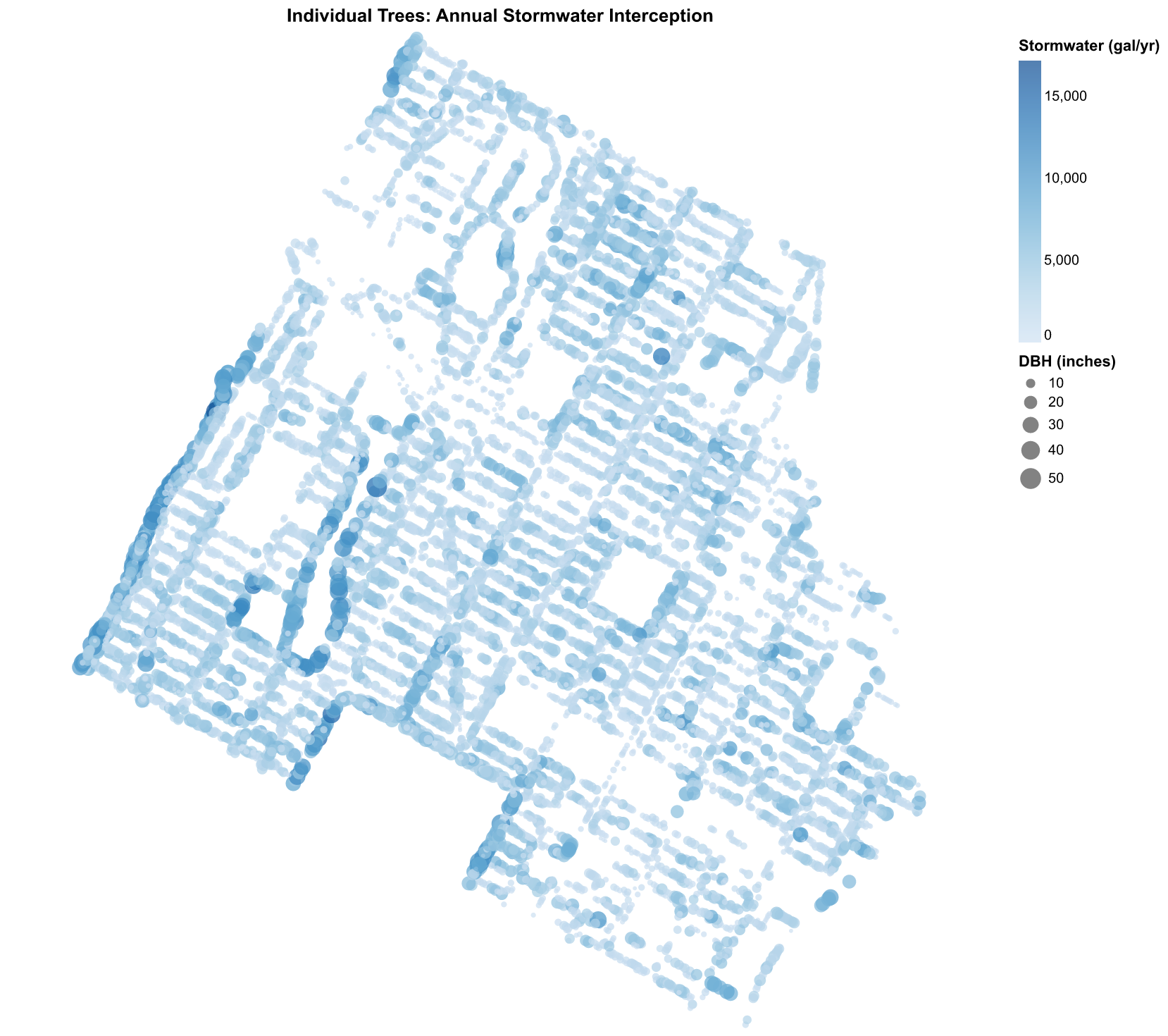
Step 6: Map individual trees colored by stormwater benefit
Before we aggregate to blocks, let's look at the per-tree data. The color encodes annual stormwater interception (gallons/year); point size encodes DBH, the same as Tutorial 2.
chart_StreetTree_Storm = alt.Chart(df_StreetTree).mark_circle().encode(
    longitude='longitude:Q',
    latitude='latitude:Q',
    color=alt.Color(
        'stormwater_gal_yr:Q',
        scale=alt.Scale(scheme='blues'),
        legend=alt.Legend(title='Stormwater (gal/yr)')
    ),
    size=alt.Size(
        'tree_dbh:Q',
        scale=alt.Scale(range=[0, 228]),
        legend=alt.Legend(title='DBH (inches)')
    ),
    tooltip=[
        alt.Tooltip('spc_common:N', title='Species'),
        alt.Tooltip('SpCode:N', title='Equations used'),
        alt.Tooltip('tree_dbh:Q', title='DBH (in)', format='.1f'),
        alt.Tooltip('stormwater_gal_yr:Q', title='Stormwater (gal/yr)', format=',.0f'),
        alt.Tooltip('co2_seq_kg_yr:Q', title='CO₂ sequestered (kg/yr)', format='.1f')
    ]
).project(
    type='mercator'
).properties(
    width=700,
    height=700,
    title='Individual Trees: Annual Stormwater Interception'
)

chart_StreetTree_Storm
Hover over a few trees. Notice how much the stormwater value varies, and that two trees of the same diameter give different numbers if they are different species.
Step 7: Spatial join to blocks and aggregate
Now we follow the exact same spatial join pattern as Tutorial 2. The only difference is that instead of just counting trees, we're also summing up benefit estimates. Here's the sequence:
- Convert the street tree dataframe to a GeoDataFrame using lat/lon
- Load the block GeoPackage
sjointhe two (keeping the structure of the street trees)groupbyblock to count trees and sum benefits- Merge back to the block GeoDataFrame for polygon geometry
# Load blocks. Same file and reprojection as Tutorial 2
gdf_Blocks = gpd.read_file('/content/nycb2010_um.gpkg').to_crs(epsg=4326)

gdf_Blocks.head()
# Convert df_StreetTree to a GeoDataFrame. Same pattern as Tutorial 2
gdf_StreetTree = gpd.GeoDataFrame(
    df_StreetTree,
    geometry=gpd.points_from_xy(df_StreetTree['longitude'], df_StreetTree['latitude']),
    crs='EPSG:4326'
)

# Spatial join: attach block ID to each tree row
gdf_joined = gpd.sjoin(gdf_Blocks, gdf_StreetTree, how='right', predicate='contains')

# Aggregate per block: count trees, sum benefits
gdf_agg = gdf_joined.groupby('BCTCB2010').agg(
    tree_count=('tree_id', 'count'),
    total_stormwater_gal=('stormwater_gal_yr', 'sum'),
    total_co2_kg=('co2_seq_kg_yr', 'sum')
).reset_index()

# Average stormwater per tree. Shows where individual trees are working hardest,
# independent of how many trees a block has
gdf_agg['stormwater_per_tree'] = gdf_agg['total_stormwater_gal'] / gdf_agg['tree_count']

# Merge aggregated values back to the block GeoDataFrame
gdf_BenefitBlocks = gdf_Blocks.merge(gdf_agg, on='BCTCB2010', how='left')

# Fill blocks with no trees with 0 rather than NaN
gdf_BenefitBlocks[['tree_count', 'total_stormwater_gal', 'total_co2_kg', 'stormwater_per_tree']] = (
    gdf_BenefitBlocks[['tree_count', 'total_stormwater_gal', 'total_co2_kg', 'stormwater_per_tree']]
    .fillna(0)
)

print(f"Blocks with at least one tree: {(gdf_BenefitBlocks['tree_count'] > 0).sum()}")
print(f"Total blocks: {len(gdf_BenefitBlocks)}")
gdf_BenefitBlocks[['BCTCB2010', 'tree_count', 'total_stormwater_gal', 'total_co2_kg', 'stormwater_per_tree']].head(10)
Step 8: Three choropleths
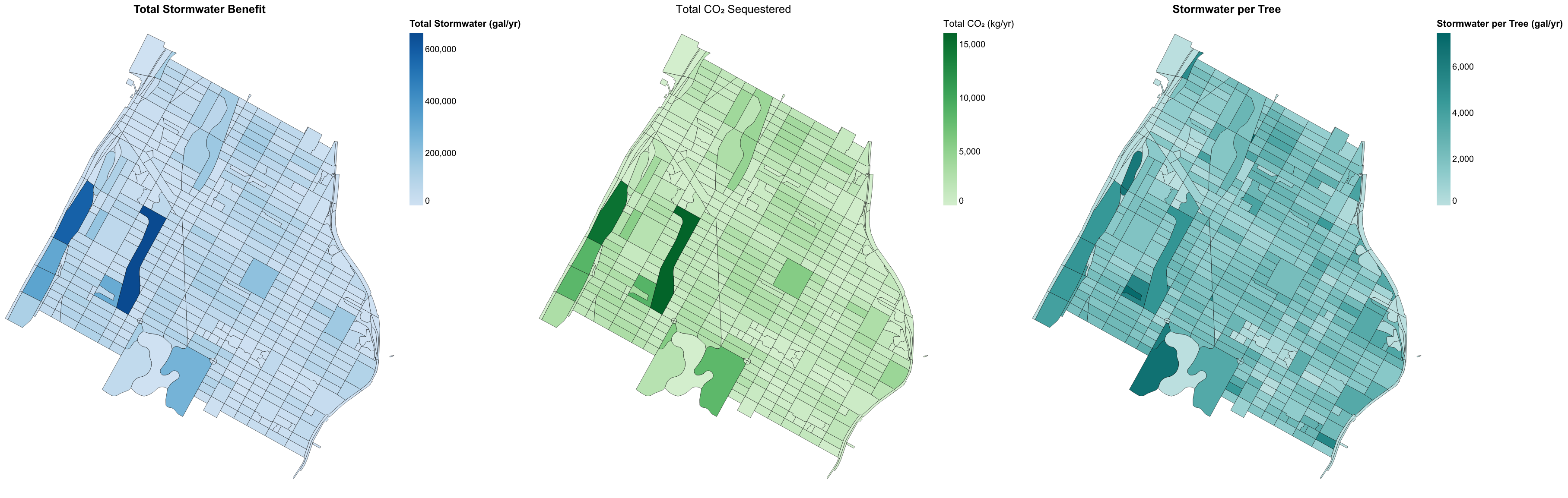
Now let's map the three aggregated metrics. The first two (total stormwater, total CO₂) show where the city gets the most ecological work done. The third, stormwater per tree, is the interesting one: it removes the effect of tree count and shows where individual trees are working hardest, regardless of how many there are.
# Shared base chart properties
base = alt.Chart(gdf_BenefitBlocks).mark_geoshape(
    stroke='black',
    strokeWidth=0.3
).project(
    type='mercator'
).properties(
    width=450,
    height=550
)

# Chart 1: Total stormwater benefit per block (blue)
chart_Stormwater = base.encode(
    color=alt.Color(
        'total_stormwater_gal:Q',
        scale=alt.Scale(scheme='blues'),
        legend=alt.Legend(title='Total Stormwater (gal/yr)')
    ),
    tooltip=[
        alt.Tooltip('BCTCB2010:N', title='Block'),
        alt.Tooltip('tree_count:Q', title='Tree Count'),
        alt.Tooltip('total_stormwater_gal:Q', title='Stormwater (gal/yr)', format=',.0f')
    ]
).properties(
    title='Total Stormwater Benefit'
)

# Chart 2: Total CO₂ sequestered per block (green)
chart_CO2 = base.encode(
    color=alt.Color(
        'total_co2_kg:Q',
        scale=alt.Scale(scheme='greens'),
        legend=alt.Legend(title='Total CO₂ (kg/yr)')
    ),
    tooltip=[
        alt.Tooltip('BCTCB2010:N', title='Block'),
        alt.Tooltip('tree_count:Q', title='Tree Count'),
        alt.Tooltip('total_co2_kg:Q', title='CO₂ (kg/yr)', format=',.0f')
    ]
).properties(
    title='Total CO₂ Sequestered'
)

# Chart 3: Stormwater per tree. Where individual trees are working hardest
chart_StormPerTree = base.encode(
    color=alt.Color(
        'stormwater_per_tree:Q',
        scale=alt.Scale(scheme='teals'),
        legend=alt.Legend(title='Stormwater per Tree (gal/yr)')
    ),
    tooltip=[
        alt.Tooltip('BCTCB2010:N', title='Block'),
        alt.Tooltip('tree_count:Q', title='Tree Count'),
        alt.Tooltip('stormwater_per_tree:Q', title='Stormwater per Tree (gal/yr)', format=',.0f')
    ]
).properties(
    title='Stormwater per Tree'
)

chart_Stormwater | chart_CO2 | chart_StormPerTree
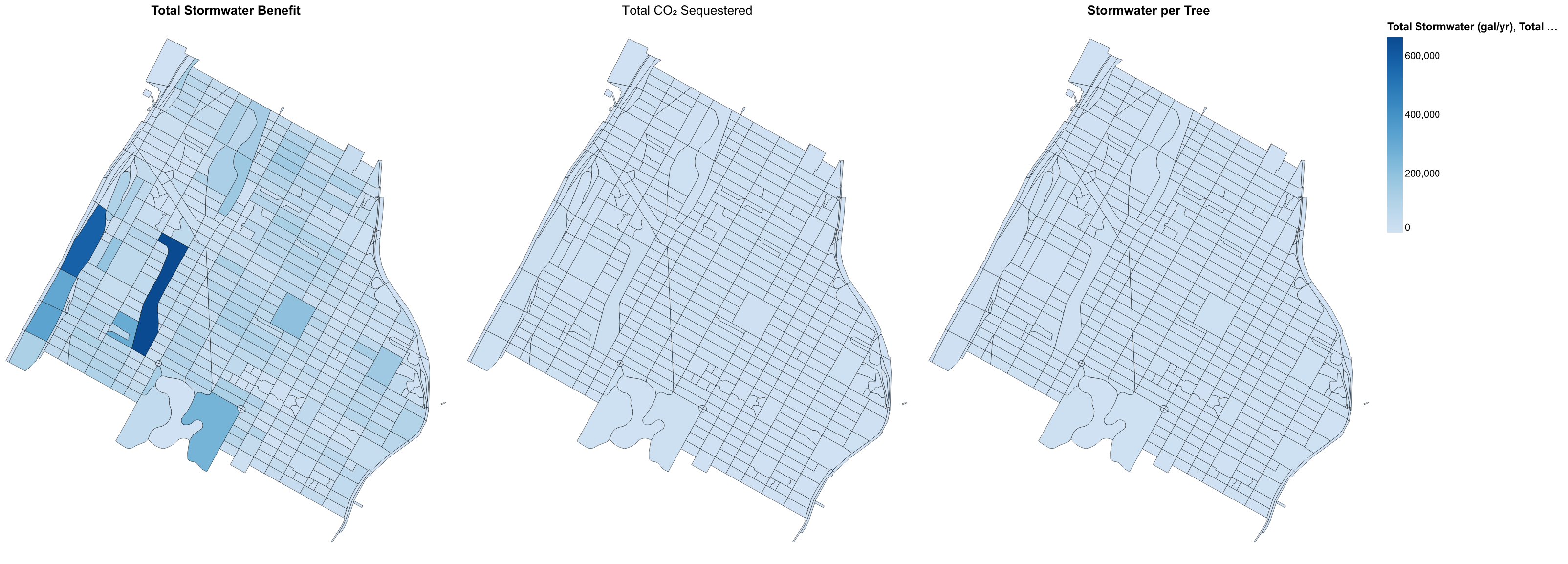
And... it didn't work! The second and third maps are almost blank. What is going on here? Look at the legend. There is only one, and it is labeled with all three fields. When you put charts side by side, Altair assumes they share a color scale, so the CO₂ map (thousands of kilograms) and the per-tree map (thousands of gallons) are being drawn on the stormwater scale (hundreds of thousands of gallons). Tell it to keep the three scales separate:
(chart_Stormwater | chart_CO2 | chart_StormPerTree).resolve_scale(color='independent')
Step 9: Reflection
If we look at the three maps, we can see a few trends emerge:
The first two maps (total stormwater, total CO₂) will tend to track the number of trees. Blocks with more trees simply generate more total benefit. Are trees evenly distributed, or do they reflect historical investment in communities?
The stormwater-per-tree map removes the effect of count. A block with a high per-tree value has large trees of species with wide crowns. A block with a low per-tree value may have many small or narrow trees. Where are the high-performing individual trees located relative to the areas that need the most infrastructure relief?
There's a broader methodological point here, in that the city provides estimates for the benefits of street trees from a similar kind of model, averaged across the whole city. This does not take into account which areas may be more or less in need of green infrastructure—rather it is a straightforward projection based on the observed physical qualities of trees, generalized by species. What would a more spatially precise model look like? A more equitable one?
Step 10: Run it forward
So far we have applied a rule to a record. In this last step we give the rule time, and make our first bona-fide simulation.
Each year, every tree grows by its species' curve, as in Step 5, but trees also die. The Northeast guide assumes 2.8% of trees die each year for their first five years and 0.57% a year after that (p. 94). Rather than removing trees at random, we keep track of the share of each tree that is still standing, and weight its benefits by that share. That way the run gives the same answer every time.
The code below recomputes stormwater for each year from 2015 to 2045. Each year, the function records the stormwater of every tree, weighted by how much of it is still standing. Then it applies the year's deaths, grows every tree by one year, and moves on.
def run(df, years=range(2015, 2046), mortality=True):
    sp = df['SpCode'].to_numpy()
    dbh_cm = df['tree_dbh'].to_numpy() * 2.54
    age = np.maximum(predict('age_from_dbh', sp, dbh_cm), 0)
    standing = np.where(np.isnan(dbh_cm), 0.0, 1.0)   # the share of each tree still standing
    rows = []
    for year in years:
        gal = stormwater_gal_yr(sp, dbh_cm)
        rows.append({'year': year, 'trees': standing.sum(), 'stormwater_gal': np.nansum(standing * gal)})
        if mortality:
            # 2.8% a year for trees under 5 years old, 0.57% after (Northeast Community Tree Guide, p. 94)
            standing = standing * np.where(age < 5, 1 - 0.028, 1 - 0.0057)
        dbh_cm = grow_one_year(sp, dbh_cm, age)
        age = age + 1
    return pd.DataFrame(rows)
Then run the baseline:
baseline = run(df_StreetTree)
baseline.tail()
With this subset, 2015 comes out at about 25.0 million gallons a year from 12,093 trees with a usable diameter, and 2045 at about 62.9 million from about 10,140 trees.
Now a second run that differs from the first by exactly one thing. Here I will turn off deaths.
no_deaths = run(df_StreetTree, mortality=False)

baseline['scenario'] = 'Northeast guide mortality'
no_deaths['scenario'] = 'no trees die'
runs = pd.concat([baseline, no_deaths])

alt.Chart(runs).mark_line().encode(
    x='year:O',
    y=alt.Y('stormwater_gal:Q', title='Stormwater intercepted (gal/yr)'),
    color='scenario:N'
).properties(width=600, height=300, title='Two runs, one changed value')
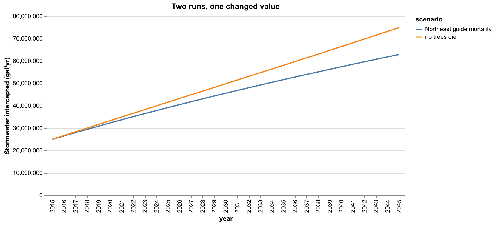
Both lines rise for thirty years because the trees keep growing and nothing is planted to replace the ones that die. There are no storms, no construction, no disease, and no planting. Everything the chart shows was put there by the equations and the numbers above.
Adding chance
Both runs above give one line each. In a statistics course, a line like this is called a point forecast: the average of everything the rule says could happen (Hyndman and Athanasopoulos, Forecasting: Principles and Practice, section 1.7).
Our standing share is exactly that kind of average. A simulation, in the statistical sense, draws the random parts of the rule at random, runs many times, and looks at how far apart the runs end up (section 5.5). In our rule, the part that should be more random, is which trees die.
As a final step, let's set that up. A tree's growth doesn't depend on chance, so we can work out each tree's stormwater for every year once, and reuse it in every run:
# Each tree's stormwater and age in every year, 2015-2045, if it survives
sp = df_StreetTree['SpCode'].to_numpy()
dbh_cm = df_StreetTree['tree_dbh'].to_numpy() * 2.54
age = np.maximum(predict('age_from_dbh', sp, dbh_cm), 0)
gal_by_year, age_by_year = [], []
for year in range(2015, 2046):
    gal_by_year.append(stormwater_gal_yr(sp, dbh_cm))
    age_by_year.append(age)
    dbh_cm = grow_one_year(sp, dbh_cm, age)
    age = age + 1
gal_by_year = np.array(gal_by_year)
age_by_year = np.array(age_by_year)
Now one random run. Each year, every living tree dies with the Northeast guide's probability. The seed sets the random numbers, so the same seed always gives the same run. which lets us total only some of the trees, which we will use in a moment.
Go ahead and copy the below into your notebook. This will run an estimate of stormwater intercepted over time 100 times and draw the middle 90% of the runs as a band, with the average run from above on top of it:
def run_random(seed, which=None):
    rng = np.random.default_rng(seed)
    alive = ~np.isnan(gal_by_year[0])
    if which is not None:
        alive = alive & which
    totals = []
    for t in range(len(gal_by_year)):
        totals.append(np.nansum(gal_by_year[t][alive]))
        death_rate = np.where(age_by_year[t] < 5, 0.028, 0.0057)
        alive = alive & (rng.random(len(alive)) >= death_rate)
    return totals

years = list(range(2015, 2046))
random_runs = pd.DataFrame([run_random(seed) for seed in range(100)], columns=years)

band = pd.DataFrame({
    'year': years,
    'low': random_runs.quantile(0.05).to_numpy(),
    'high': random_runs.quantile(0.95).to_numpy(),
})

chart_Band = alt.Chart(band).mark_area(opacity=0.3).encode(
    x='year:O',
    y=alt.Y('low:Q', title='Stormwater intercepted (gal/yr)'),
    y2='high:Q'
)
chart_Average = alt.Chart(baseline).mark_line(color='black').encode(x='year:O', y='stormwater_gal:Q')

(chart_Band + chart_Average).properties(width=600, height=300, title='100 random runs and the average run')
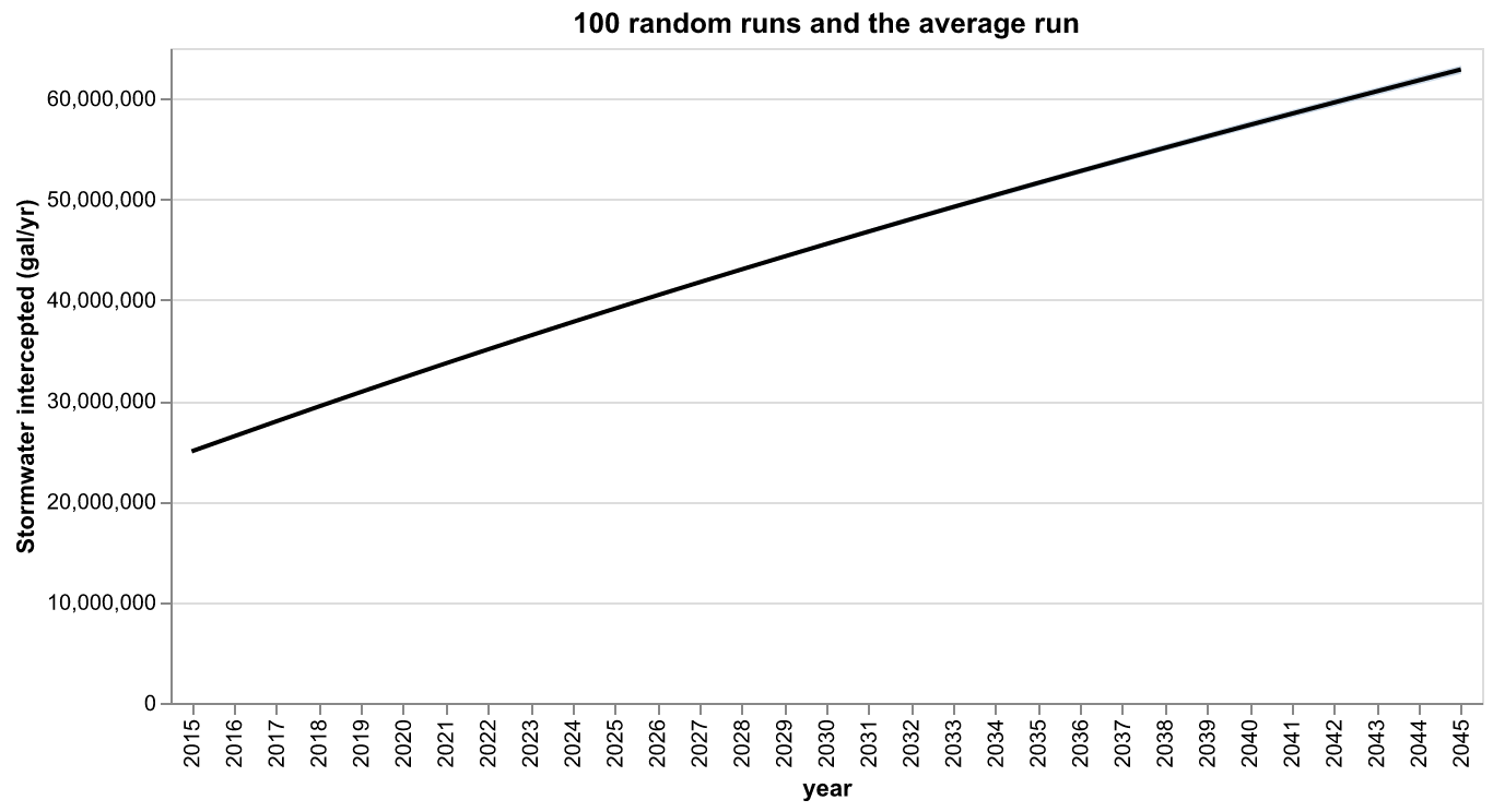
You will have to look closely to see the band at all. In 2045, 90% of the runs fall between 62.4 and 63.3 million gallons, around an average of 62.9 million. Across 12,000 trees and a large area, the trees that happen to die in one run are balanced by the ones that happen to survive.
A single block is different. Here is one block of 11 trees, bounded by East 130th and East 131st Streets and Park and Lexington Avenues, and with every run drawn as its own line.:
# The block each tree is in, from the spatial join in Step 7.
tree_block = gdf_joined['BCTCB2010'].groupby(level=0).first().reindex(df_StreetTree.index).to_numpy()

# A filter to narrow down the trees to just one block.
one_block = (tree_block == '10242001004')

# 100 random runs that total only this block's trees.
block_runs = pd.DataFrame([run_random(seed, which=one_block) for seed in range(100)], columns=years)

# The spread of the 100 runs in 2045: the lowest, the 5th, 50th and 95th percentiles, and the highest
print(block_runs[2045].describe(percentiles=[0.05, 0.5, 0.95]))

# Altair wants one row per run per year, so turn the wide table into a long one
block_long = block_runs.reset_index(names='run').melt(id_vars='run', var_name='year', value_name='stormwater_gal')

# One faint line per run. detail='run:N' draws a separate line for each run without giving each its own color
chart_BlockRuns = alt.Chart(block_long).mark_line(opacity=0.15).encode(
    x='year:O',
    y=alt.Y('stormwater_gal:Q', title='Stormwater intercepted (gal/yr)'),
    detail='run:N'
).properties(width=600, height=300, title='One block, 100 random runs')

chart_BlockRuns
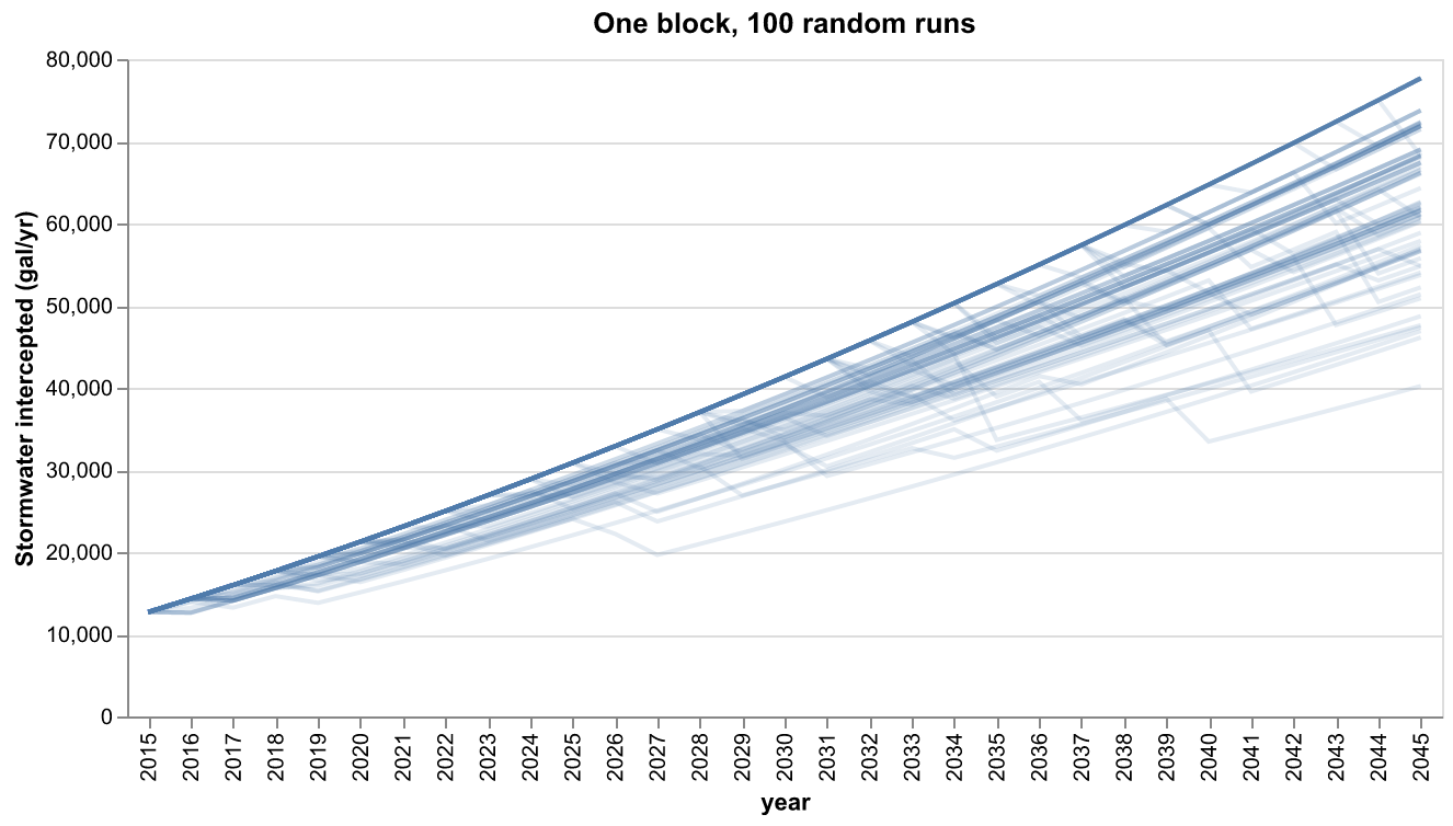
In this block, 90% of the runs fall between about 48,700 and 77,700 gallons in 2045, and the worst run is 40,200. The top of that range, 77,700, is the run where no tree in the block dies. Whether two or three of its larger trees survive makes a large difference, and the average line hides that. Try a block of your own.
So with that, you have made your first proper simulation in the statistical sense, a Monte Carlo simulation: the same rule, run many times with its random part drawn fresh each time. Note that it doesn't cover doubt about the rule itself: If the right interception figure were the cork oak's 27% rather than the pear's 15%, every tree would catch 80% more rain, and no number of runs would show it.
How close is this to Parks' numbers?
The Parks Department publishes its stormwater figure for every tree on the Tree Map (the Eco Benefits table on NYC Open Data, last built in 2022). Here are ten trees from our subset, matched to Parks' records by location and species. Parks' trunk diameters were measured later than the census, so both columns use Parks' diameter.
| Tree | Species | DBH (in) | Our rule (gal/yr) | Parks (gal/yr) |
|---|---|---|---|---|
| 608 West 139th St | green ash | 9 | 2,054 | 938 |
| 256 West 136th St | ginkgo | 8 | 826 | 468 |
| 73 East 118th St | Callery pear | 10 | 1,901 | 2,031 |
| 127 West 136th St | Callery pear | 26 | 12,015 | 3,720 |
| 62 West 119th St | pin oak | 14 | 3,513 | 1,667 |
| 471 Central Park West | pin oak | 37 | 14,984 | 7,122 |
| 75 West 115th St | northern red oak | 13 | 2,872 | 822 |
| 325 East 118th St | littleleaf linden | 11 | 2,199 | 616 |
| 2 West 106th St | Japanese zelkova | 11 | 2,830 | 959 |
| 1 Hamilton Terrace | Japanese zelkova | 26 | 8,236 | 4,663 |
How did we do? Not so great. Only the 10-inch Callery pear comes out close. For the other nine, our number is about two to three and a half times Parks'. I don't know for certain which part of our rule is responsible. The 15% from two trees in Davis is the step that differs most from i-Tree, so it is the first place I would look. Parks' numbers also come in steps: trees of the same size often get exactly the same figure, which suggests that i-Tree Streets works in diameter classes rather than tree by tree.
Assignment 3
Think of a forecast (or a hindcast) that could come out of the dataset you used for Assignment 2, and sketch out it's rule and run. No code. Details on the assignment page.
Module by Adam Vosburgh, Spring 2026. Updated for Colab, with Step 10 added, Fall 2026. Revised to follow i-Tree Streets and the Urban Tree Database, September 2026.